Introduction
Sentiment analysis is a fundamental task in natural language processing (NLP) that focuses on identifying the emotional tone behind textual data. From product reviews and social media posts to movie critiques, understanding sentiment helps businesses and researchers extract meaningful insights from large volumes of text. One of the most commonly used benchmark datasets for this task is the IMDB movie reviews dataset, which contains labeled positive and negative reviews.
Recurrent Neural Networks (RNNs) have traditionally been a popular choice for sentiment analysis because they are designed to handle sequential data such as text. However, standard RNNs often struggle with long-term dependencies, which led to the development of improved architectures like Long Short-Term Memory (LSTM) and Gated Recurrent Unit (GRU) networks.
In this blog, we conduct a comparative study between a Vanilla RNN and a Long Short-Term Memory (LSTM) network for sentiment classification on the IMDB dataset. The goal is not only to compare performance metrics but also to understand how a standard RNN behaves during training, identify its practical limitations, and observe how LSTM addresses these shortcomings through its gated memory mechanism. Through this comparison, we highlight the strengths, weaknesses, and real-world trade-offs between these two sequential models.
Why Sentiment Analysis with RNNs?
Text data is inherently sequential. The meaning of a word often depends on the words that come before it, making sequence modeling essential for NLP tasks. RNNs are specifically designed to process sequences by maintaining a hidden state that captures information from previous time steps.
For sentiment analysis, this sequential modeling capability allows RNN-based models to understand context, negations, and dependencies across words in a sentence or paragraph. For example, phrases like “not good” or “although the movie started slow, it ended brilliantly” require contextual understanding that simple bag-of-words models often fail to capture.
Despite newer architectures like Transformers gaining popularity, RNN-based models remain important for understanding the evolution of sequence modeling and for use cases where computational resources are limited.
IMDB Dataset Overview
The IMDB dataset is a widely used benchmark for binary sentiment classification. It consists of movie reviews labeled as either positive or negative, making it ideal for evaluating text classification models.
Dataset Characteristics
-
Task: Binary sentiment classification (positive / negative)
-
Total reviews: 50,000
-
Training set: 25,000 reviews
-
Test set: 25,000 reviews
-
Balanced classes: Equal number of positive and negative samples
Preprocessing Steps
Common preprocessing steps applied to the IMDB dataset include:
-
Text tokenization
-
Converting words into integer indices
-
Limiting vocabulary size
-
Padding or truncating sequences to a fixed length
These steps ensure that the text data can be efficiently processed by neural network models.
Recurrent Neural Network Architectures
This section provides a high-level overview of the RNN architectures – Vanilla RNN and LSTM compared in this study.
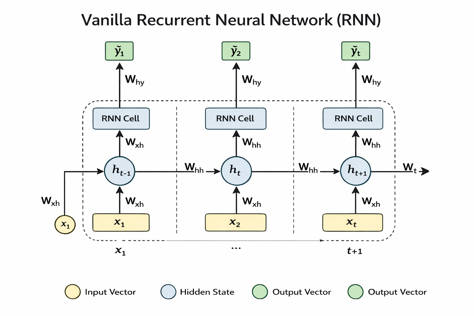
Vanilla RNN
The Vanilla RNN is the simplest form of recurrent neural network. It processes sequences by updating a hidden state at each time step using the current input and the previous hidden state.
Advantages:
Simple and easy to implement
Fewer parameters
Useful for short sequences
Limitations:
Suffers from the vanishing gradient problem
Struggles with long-term dependencies
Performance degrades on longer text sequences
Because IMDB reviews can be lengthy, vanilla RNNs often fail to retain important contextual information from earlier parts of the review.
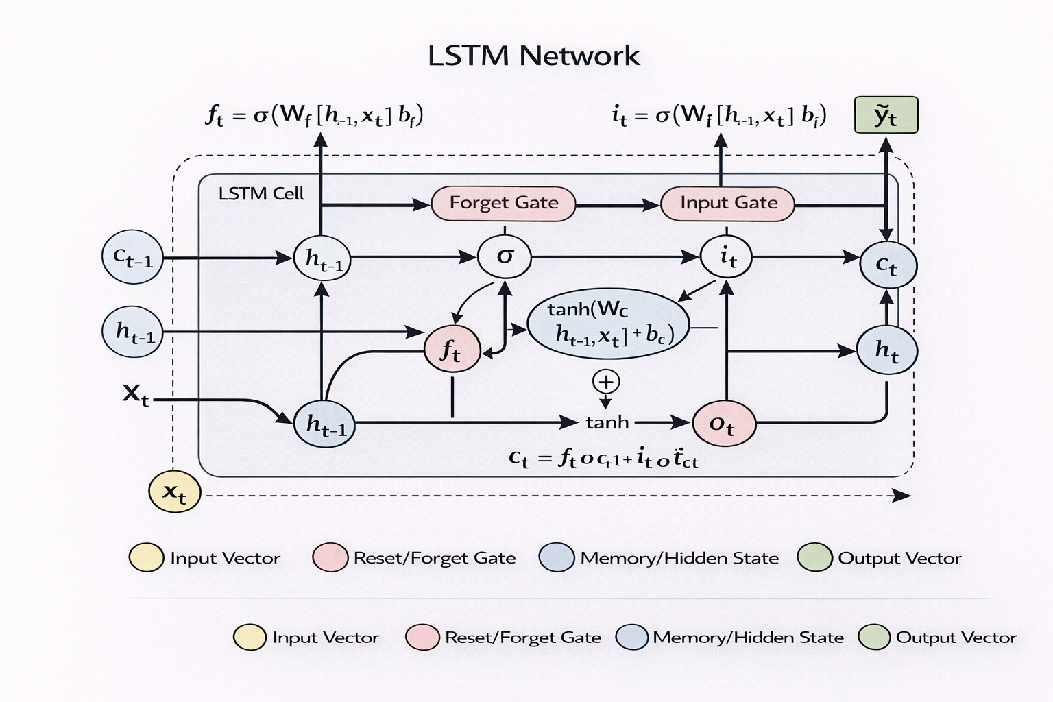
Long Short-Term Memory (LSTM)
LSTM networks were introduced to overcome the limitations of vanilla RNNs. They use a gated architecture that controls the flow of information through the network.
Key components of LSTM include:
Forget gate
Input gate
Output gate
Cell state
These mechanisms allow LSTMs to selectively remember or forget information over long sequences.
Advantages:
Excellent at capturing long-term dependencies
Stable training behavior
Strong performance on text-based tasks
Limitations:
Computationally expensive
Larger number of parameters
Slower training compared to simpler models
Want to learn more about RNN and LSTM architecture ? Read our detailed guide explaining how Recurrent Neural Networks (RNN) and Long Short-Term Memory (LSTM) models work.
Experimental Setup
To ensure a fair and controlled comparison between Vanilla RNN and LSTM, both the models were trained under identical experimental conditions. The only difference between experiments was the recurrent unit type. This controlled design allows performance differences to be attributed solely to architectural variations.
Dataset Split
The IMDb dataset consists of 50,000 labeled reviews, evenly split into:
25,000 training samples
25,000 test samples
From the training set, a validation subset was created to monitor generalization performance and enable early stopping. The test set was used strictly for final evaluation and was not accessed during training.
Model Configuration
Both RNN and LSTM models were configured with identical hyperparameters:
Vocabulary Size: 20,000
Embedding Dimension: 200
Hidden Size: 128
Number of Layers: 1
Direction: Unidirectional
Dropout: 0.5
Output Dimension: 1 (Binary classification)
This ensures architectural fairness across experiments.
Training Configuration
-
Loss Function: Binary Cross Entropy with Logits (BCEWithLogitsLoss)
-
Optimizer: Adam
-
Learning Rate: 0.001
-
Weight Decay: 1e-4
-
Batch Size: 128
-
Early Stopping: Based on validation loss
The models output raw logits, which are passed directly to BCEWithLogitsLoss. Sigmoid activation is applied only during evaluation for probability estimation.
Regularization Strategy
To improve generalization and prevent overfitting:
Dropout (0.5) was applied before the final classification layer.
L2 regularization was implemented through weight decay in the optimizer.
Early stopping was employed to halt training when validation performance stopped improving.
Evaluation Metrics
Model performance was evaluated using:
Training Loss
Validation Loss
Training Accuracy
Validation Accuracy
Final Test Accuracy
Binary predictions were obtained by applying a sigmoid function to logits and thresholding at 0.5.
Implementation Details
This section describes the technical implementation, including data preprocessing, model construction, and training workflow.
Data Preparation
Effective sentiment modeling begins with structured and consistent text preprocessing. Since neural networks operate on numerical tensors rather than raw text, the IMDb reviews were transformed into model-ready sequences through a carefully designed preprocessing pipeline.
1. Text Normalization and Tokenization
A lightweight custom tokenizer was implemented to standardize input text before numerical encoding.
 def simple_tokenize(text):
    text = text.lower()
    text = re.sub(r'[^a-z0-9\s]', '', text)
    return text.split()
This tokenizer performs three key operations:
Lowercasing – All text is converted to lowercase to reduce vocabulary size and avoid treating words like “Movie” and “movie” as separate tokens.
Character Filtering – A regular expression removes all non-alphanumeric characters except whitespace. This eliminates punctuation and special symbols that are unlikely to contribute meaningfully to binary sentiment classification.
Whitespace Tokenization – The cleaned text is split on spaces to produce word-level tokens.
Although simple, this approach is effective for baseline sentiment analysis tasks and maintains computational efficiency without introducing external dependencies.
2. Vocabulary Construction
A vocabulary was built from the training dataset only to prevent data leakage. Tokens were ranked by frequency, and the top 20,000 most frequent words were retained.
Two special tokens were introduced:
-
<PAD> (index 0) — used for sequence padding
-
<UNK> — used to represent out-of-vocabulary words
Limiting vocabulary size improves training efficiency and reduces noise introduced by rare terms.
3. Integer Encoding
Each token was mapped to its corresponding index in the vocabulary dictionary (word_to_idx).
This transforms text into sequences of integers suitable for embedding lookup.
4. Sequence Length Analysis
Movie reviews in the IMDb dataset vary significantly in length. Instead of selecting an arbitrary truncation threshold, the distribution of review lengths was analyzed.
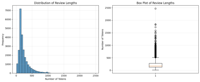
Based on this distribution, selected max_length: 595
This value corresponds to approximately the 95th percentile of review lengths, meaning that 95% of all reviews fall within this length.
Choosing the 95th percentile provides a balanced trade-off:
Preserves most contextual information
Prevents excessive padding
Controls memory usage
Improves training efficiency
5. Padding and Truncation Strategy
To ensure consistent batch processing:
-
Sequences shorter than 595 tokens were padded using <PAD> (index 0).
-
Sequences longer than 595 tokens were truncated to 595 tokens.
6. Handling Variable-Length Sequences
To prevent padded tokens from influencing hidden state updates, pack_padded_sequence() was used before passing inputs to the recurrent layer.
This improves:
-
Computational efficiency
-
Gradient flow
-
Model stability
The original sequence lengths were passed alongside the padded inputs.
Model Architecture Implementation
This section describes the implementation of the sentiment classification models used in the experiments. Both architectures follow a similar pipeline consisting of an embedding layer, a recurrent sequence modeling layer, a dropout regularization layer, and a fully connected output layer. The primary difference between the two models lies in the type of recurrent unit used: a Vanilla RNN or an LSTM.
The models are implemented using the PyTorch deep learning framework.
Overall Model Pipeline
The sentiment classification model follows the following processing pipeline:
Tokenized Review → Embedding Layer → Recurrent Layer (RNN/LSTM) → Dropout → Fully Connected Layer → Output Logits
The final output represents the predicted sentiment score for each review.
1. Embedding Layer
The first layer of the model is an embedding layer that converts token indices into dense vector representations.
self.embedding = nn.Embedding(vocab_size, embedding_dim, padding_idx=0)
Configuration –
-
Vocabulary size: 20,000
-
Embedding dimension: 200
-
Padding index: 0
Purpose –
Text input to the model is represented as integer indices corresponding to words in the vocabulary. However, neural networks cannot directly interpret these indices as meaningful representations. The embedding layer addresses this by mapping each word index to a dense vector in a continuous vector space.
Instead of representing words using sparse one-hot vectors, embeddings allow the model to learn semantic relationships between words during training. Words that appear in similar contexts often develop similar vector representations.
For example, words such as “excellent”, “amazing”, and “fantastic” may eventually occupy nearby positions in the embedding space.
The padding_idx=0 parameter ensures that padding tokens used for sequence alignment do not contribute to gradient updates during training.
2. Recurrent Sequence Modelling Layer
After the embedding layer, the sequence of word vectors is passed to a recurrent neural network layer that processes the review sequentially.
Two variants were implemented:
Vanilla RNN
LSTM
Both layers operate on sequences of embeddings and update hidden states as they process each token in the sequence.
a. Vanilla RNN Layer
The Vanilla RNN model uses the following configuration:
 self.rnn = nn.RNN(
    input_size=embedding_dim,
    hidden_size=hidden_size,
    num_layers=1,
    nonlinearity="tanh",
    batch_first=True
)
Configuration –
-
Input size: 200
-
Hidden size: 128
-
Number of layers: 1
-
Activation function: tanh
-
Batch-first format: True
Working Mechanism –
At each time step, the RNN updates its hidden state using the current input embedding and the previous hidden state.
The update rule can be expressed as:
Where:
xt is the input embedding at time step t
ht−1 is the previous hidden state
ht is the updated hidden state
As the network processes the review token by token, the hidden state gradually accumulates contextual information about the sequence.
After the entire sequence has been processed, the final hidden state is used as the representation of the entire review.
b. LSTM Layer
The LSTM model replaces the vanilla RNN layer with an LSTM layer.
 self.lstm = nn.LSTM(
    input_size=embedding_dim,
    hidden_size=hidden_size,
    batch_first=True
)
Configuration –
-
Input size: 200
-
Hidden size: 128
-
Single-layer LSTM
-
Unidirectional processing
Working Mechanism –
Unlike vanilla RNNs, LSTMs maintain two states:
-
Hidden state (ht)
-
Cell state (ct)
The cell state acts as a long-term memory that allows the network to preserve information over long sequences.
LSTMs use three gating mechanisms to control information flow:
Forget Gate – Determines which information should be discarded from the cell state.
Input Gate – Controls which new information should be added to the cell state.
Output Gate – Determines which parts of the cell state should influence the hidden state output.
These gates enable LSTMs to capture long-term dependencies in text sequences and significantly mitigate the vanishing gradient problem that affects vanilla RNNs.
3. Dropout Regularization
Before classification, dropout is applied to the final hidden representation.
self.dropout = nn.Dropout(0.5)
Dropout randomly disables 50% of neurons during training, which helps reduce overfitting and improves model generalization.
4. Fully Connected Output Layer
The final layer of the model is a fully connected linear layer.
self.fc = nn.Linear(hidden_size, 1)
This layer maps the hidden representation to a single scalar value representing the predicted sentiment score.
The model outputs raw logits, which are passed directly to the loss function.
Loss Function and Output Handling
The models return raw logits.
BCEWithLogitsLoss() internally applies sigmoid activation and computes binary cross-entropy in a numerically stable manner as follows :
Optimization Strategy
The Adam optimizer was selected due to its adaptive learning rate mechanism and strong empirical performance in NLP tasks.
Weight decay (1e-4) was applied to introduce L2 regularization and reduce overfitting.
optimizer = torch.optim.Adam(model.parameters(), lr=0.001,weight_decay=1e-4)
Model Capacity
Vanilla RNN Total Parameters: 4,042,369
LSTM Total Parameters: 4,169,089
The majority of parameters originate from the embedding matrix (20,000 × 200), which dominates the model’s representational capacity.
The LSTM architecture contains more parameters due to its gated structure, increasing model complexity and learning capacity.
Results and Comparative Analysis
This section presents the experimental results obtained from training Recurrent Neural Network (RNN) and Long Short-Term Memory (LSTM) models for sentiment classification on movie reviews. The models were evaluated using validation loss, test accuracy, and predictions on custom review samples to assess both quantitative performance and qualitative behavior.
Vanilla RNN Results
Training Performance
- Early Stopping Triggered: Epoch 19
- Best Validation Loss: 0.5234 (Epoch 9)
The model achieved optimal generalization relatively early during training, after which validation performance began to plateau.
Test Performance
- Test Loss: 0.5173
- Test Accuracy: 75.94%
Although the Vanilla RNN successfully learned sentiment patterns, its performance indicates limitations in handling long contextual dependencies.
Qualitative Evaluation — Custom Reviews
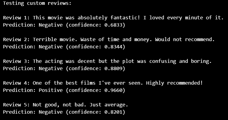
| Review | Prediction | Confidence | Observation |
|---|---|---|---|
| Fantastic movie |  Negative Negative | 0.6833 | Misclassification |
| Terrible movie |  Negative Negative | 0.8344 | Correct |
| Confusing plot | Negative | 0.8809 | Correct |
| Best films ever | Positive | 0.9660 | Correct |
| Average movie | Negative | 0.8201 | Reasonable |
Analysis
The RNN incorrectly classified a strongly positive review as negative. This behavior highlights a known limitation of traditional RNNs:
Difficulty preserving long-range sentiment cues
Sensitivity to earlier tokens in sequences
Gradual information decay during sequence processing
The model tends to rely heavily on localized patterns instead of overall contextual meaning.
LSTM Results
Training Performance
Early stopping triggered: Epoch 20
Best validation loss: 0.3661 (Epoch 10)
The significantly lower validation loss demonstrates improved learning stability compared to the Vanilla RNN.
Test Performance
Test Loss: 0.3677
Test Accuracy: 84.34%
The LSTM achieved an accuracy improvement of approximately 8.4% over the Vanilla RNN.
Qualitative Evaluation — Custom Reviews
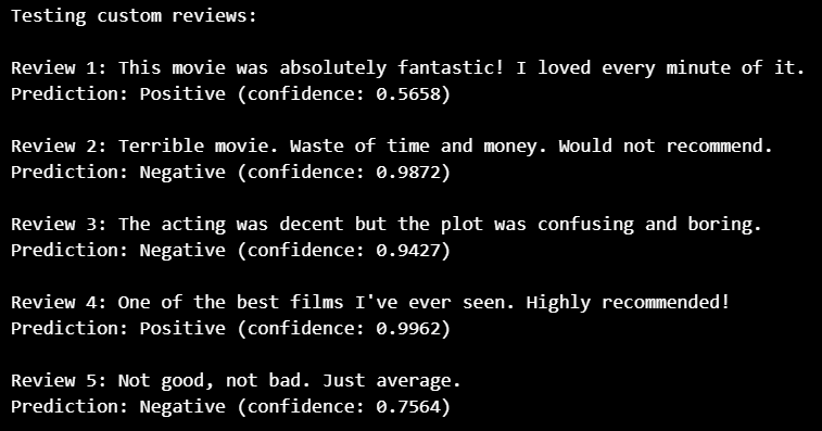
| Review | Prediction | Confidence | Observation |
|---|---|---|---|
| Fantastic movie | ✅ Positive | 0.5658 | Correct |
| Terrible movie | ✅ Negative | 0.9872 | Correct |
| Confusing plot | ✅ Negative | 0.9427 | Correct |
| Best films ever | ✅ Positive | 0.9962 | Correct |
| Average movie | ✅ Negative | 0.7564 | Correct |
Analysis
Unlike the Vanilla RNN, the LSTM correctly classified all custom reviews. This demonstrates its superior ability to understand contextual sentiment across entire sequences.
Even when confidence values were moderate, predictions remained semantically accurate, indicating better internal representation learning.
Quantitative Comparison
| Metric | Vanilla RNN | LSTM |
|---|---|---|
| Best Validation Loss | 0.5234 | 0.3661 |
| Test Loss | 0.5173 | 0.3677 |
| Test Accuracy | 75.94% | 84.34% |
| Training Stability | Moderate | High |
| Long Context Understanding | Limited | Strong |
Practical Implications
The experimental results suggest:
Vanilla RNNs are suitable as baseline models.
LSTMs provide significantly better performance for real-world sentiment analysis tasks.
Interactive Model Deployment (Streamlit App)
To make the models accessible for real-time experimentation, an interactive web application is being developed using Streamlit.
The application will allow users to:
Enter custom movie reviews
Select a trained model (RNN or LSTM)
View sentiment predictions instantly
Observe prediction confidence scores
This deployment bridges the gap between research experimentation and real-world usability by enabling anyone to test the trained models directly through a web interface.
The Streamlit application link is provided below:
Source Code and Reproducibility
To ensure transparency and reproducibility, the complete implementation used in this study is publicly available. The repository contains a Jupyter Notebook that documents the entire development process step by step.
Readers interested in exploring the implementation details or reproducing the experiments can access the full project below:
👉 GitHub Repository:
View the Complete Notebook and Source Code
The notebook provides a hands-on walkthrough of the entire workflow, from raw text processing to model evaluation, making it suitable for both learning and experimentation.
Conclusion
In this project, we explored sentiment analysis using recurrent neural network architectures on the IMDB movie review dataset, progressing from a basic Vanilla RNN to Long Short-Term Memory (LSTM) model. The goal was not only to build accurate classifiers but also to understand how different sequence modeling architectures handle textual data and long-range dependencies.
The Vanilla RNN served as an important baseline, demonstrating how sequential neural networks can learn sentiment patterns from text. While it achieved reasonable performance with a test accuracy of 75.94%, qualitative analysis revealed its limitations in preserving contextual information across long reviews. Misclassifications in strongly positive sentences highlighted the challenges caused by vanishing gradients and limited memory retention.
The LSTM model addressed these shortcomings through its gating mechanisms, enabling selective memory retention and improved contextual understanding. This architectural improvement translated into a significant performance gain, achieving 84.34% test accuracy along with lower validation and test loss. The LSTM consistently produced more reliable predictions and successfully handled nuanced sentiment expressions present in real-world reviews.
Beyond model training, this project emphasized the complete machine learning workflow — including data preprocessing, tokenization, sequence padding, architecture design, experimental evaluation, and deployment considerations. By building an interactive Streamlit application, the models were extended from research experimentation to practical usability, allowing users to test sentiment predictions on their own inputs in real time.
Overall, the experiments demonstrate a key insight in natural language processing: model architecture plays a crucial role in capturing linguistic context. While simple RNNs provide foundational understanding, gated recurrent models like LSTM offer substantial improvements for tasks involving long textual sequences.
This work highlights how deep learning models evolve from theoretical concepts into deployable intelligent systems, forming a strong foundation for further exploration into modern NLP architectures such as GRUs, attention mechanisms, and Transformer-based models.